Hello World, Quantum Computing
I kept reading that qbits can represent \(2^n\) states simultaneously, and I kept nodding along. Then I asked myself three questions and couldn't answer any of them.
- Q1. Can't n classical bits also represent \(2^n\) states? Three bits give you 000, 001, 010, 011, 100, 101, 110, 111 -- that's eight states.
- Q2. The quantum world is governed by the uncertainty principle, so how does a quantum computer actually perform computations, and how does this reduce computational cost?
- Q3. What exactly does it mean for qbits to be entangled?
Plain language kept giving me hand-wavy answers. The math turned out to be simpler than I expected.
The video is over an hour, so what follows is my reorganization of
the material -- a Hello World! for the quantum world.
A quantum computer can solve in one query what takes a classical computer two. The Deutsch-Jozsa problem shows why. To get there, we need qbits, matrix operations, and a few logic gates.
Basics
Qbit
A qbit is the fundamental unit of quantum computation. It always satisfies the following condition:
A qbit, represented by \(\begin{pmatrix} \alpha \\ \beta \end{pmatrix}\) where \(\alpha\) and \(\beta\) are complex numbers must be constrained by the equation \(||\alpha||^2 + ||\beta||^2 = 1\)
So the following are all valid qbits:
\[ \begin{pmatrix} \frac{1}{\sqrt{2}} \\ \frac{1}{\sqrt{2}} \end{pmatrix} \hspace{10pt} \begin{pmatrix} \frac{1}{2} \\ \frac{\sqrt{3}}{2} \end{pmatrix} \hspace{10pt} \begin{pmatrix} 1 \\ 0 \end{pmatrix} \hspace{10pt} \begin{pmatrix} 0 \\ -1 \end{pmatrix} \]
The basis vectors for all of these, \(\begin{pmatrix} 1 \\0 \end{pmatrix}\) and \(\begin{pmatrix} 0 \\ 1 \end{pmatrix}\), are given the special notation \(\mid 0\rangle\) and \(\mid 1\rangle\), respectively.
Superposition
This is the property you always hear about when people discuss qbits. It's often described as "being 0 and 1 at the same time," but a more precise description is: "When we measure a qbit, it collapses to an actual value of 0 or 1."
Let's take one of the qbit vectors from above as an example.
\[\begin{pmatrix} \frac{1}{\sqrt{2}} \\ \frac{1}{\sqrt{2}} \end{pmatrix}\]
This qbit has a \(\frac{1}{2}\) ( \(= || \frac{1}{\sqrt{2}} || ^2\)) probability of collapsing to either \(0\) or \(1\).
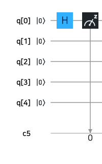
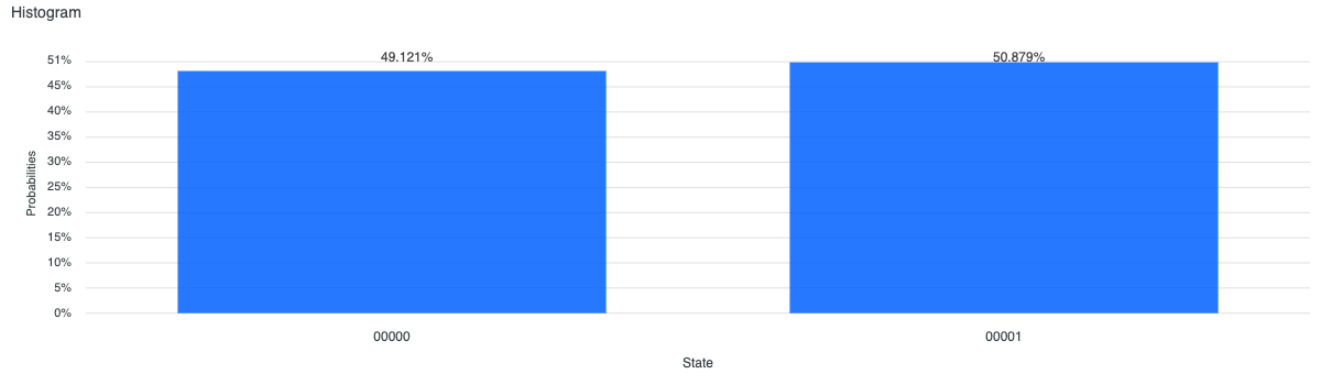
Thankfully, IBM has made their quantum computers accessible via an API. If we create this qbit there and measure it 1024 times, we can confirm that 0 and 1 each appear about 50% of the time.
\(\begin{pmatrix} \frac{1}{2} \\ \frac{\sqrt{3}}{2} \end{pmatrix}\) is a qbit with a \(\frac{1}{4}\) probability of collapsing to \(0\) and a \(\frac{3}{4}\) probability of collapsing to \(1\).
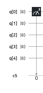
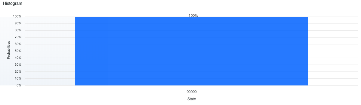
\(|0\rangle\) always collapses to 0.
Tensor product
To represent multiple qbits, we need the concept of the tensor product. The notation works like this:
\[ \binom{x_0}{x_1} \otimes \binom{y_0}{y_1} = \begin{pmatrix} x_0 \binom{y_0}{y_1} \\ x_1 \binom{y_0}{y_1} \end{pmatrix} = \begin{pmatrix} x_0 y_0 \\ x_0 y_1 \\ x_1 y_0 \\ x_1 y_1 \end{pmatrix} \]
Using this, we can represent 2 or 3 qbits as vectors.
\[ |01\rangle = \binom{1}{0} \otimes \binom{0}{1} = \begin{pmatrix} 0 \\ 1 \\ 0 \\ 0 \end{pmatrix} \hspace{10pt} |100\rangle = \binom{0}{1} \otimes \binom{1}{0} \otimes \binom{1}{0} = \begin{pmatrix} 0\\ 0\\0\\0 \\ 1 \\ 0 \\ 0 \\ 0 \end{pmatrix} \]
A vector expressed as the result of a tensor product is called a product state. From this, we can see that the product state of \(n\) qbits has size \(2^n\). If we have the following multi-qbit state: \( \binom{\frac{1}{\sqrt{2}}}{\frac{1}{\sqrt{2}}} \otimes \binom{\frac{1}{\sqrt{2}}}{\frac{1}{\sqrt{2}}} = \begin{pmatrix} \frac{1}{2} \\ \frac{1}{2} \\ \frac{1}{2} \\ \frac{1}{2} \end{pmatrix} \) then the probabilities of collapsing to \(\mid 00\rangle\), \(\mid 01\rangle\), \(\mid 10\rangle\), and \(\mid 11\rangle\) are each \(\frac{1}{4}\), meaning it can represent all four states simultaneously. In other words, when people say qbits can represent \(2^n\) states unlike classical bits, they're comparing the maximum number of states that can be held simultaneously. A classical bit can never be in more than one state at a time, so it can only process one piece of information per operation.
Another important property of product states -- one that distinguishes them from entanglement, which we'll cover later -- is that they can be factored into independent states.
The product state of multiple qbits satisfies the same constraint as a single qbit.
\[ \binom{a}{b} \otimes \binom{c}{d} = \begin{pmatrix} ac \\ ad \\ bc \\ bd \end{pmatrix} \]
\[ \text{where, } ||ac||^2 + ||ad||^2 + ||bc||^2 + ||bd||^2 = 1 \]
1-bit operations
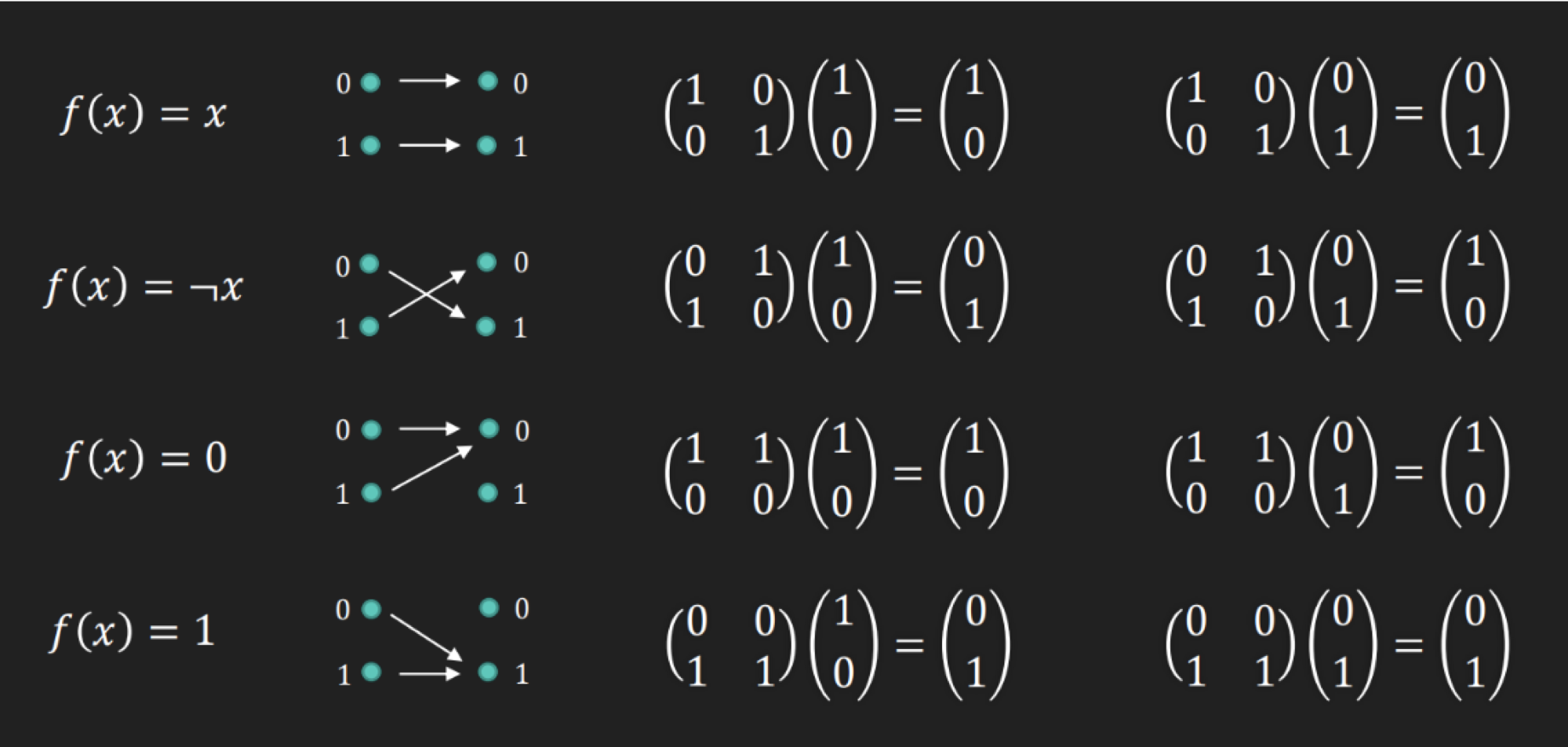
There are exactly four possible 1-bit operations: Identity, Negation, Constant-0, and Constant-1.
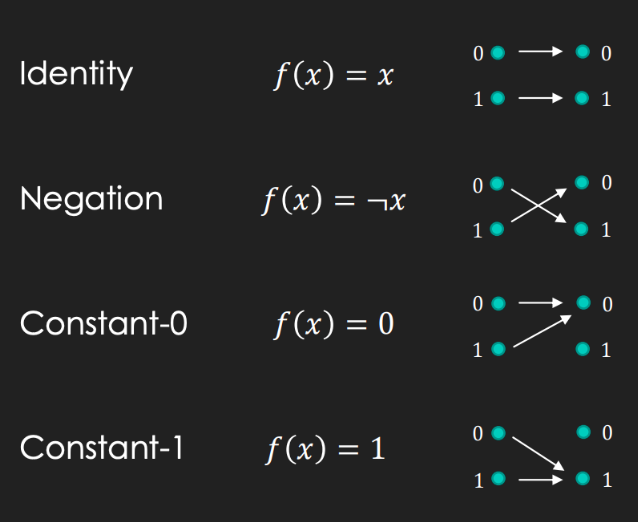
Each operation can be represented as a matrix.
\[ \text{Identity} = \begin{pmatrix} 1 & 0 \\ 0 & 1 \end{pmatrix} \] \[ \text{Negation} = \begin{pmatrix} 0 & 1 \\ 1 & 0 \end{pmatrix} \] \[ \text{Constant-0} = \begin{pmatrix} 1 & 1 \\ 0 & 0 \end{pmatrix} \] \[ \text{Constant-1} = \begin{pmatrix} 0 & 0 \\ 1 & 1 \end{pmatrix} \]
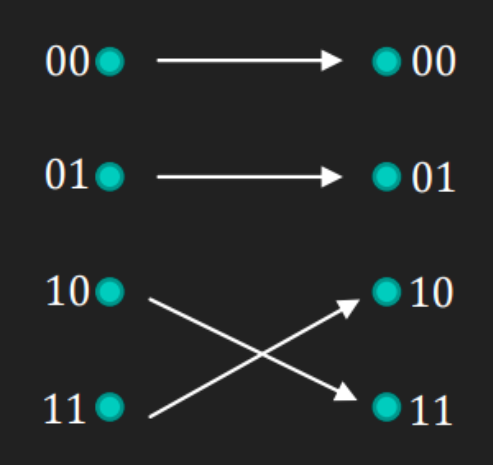
CNOT (one of the 2-bit operations)
The CNOT operation takes two bits -- a control bit and a target bit. If the control bit is 0, the target bit stays unchanged. If the control bit is 1, the target bit is flipped.
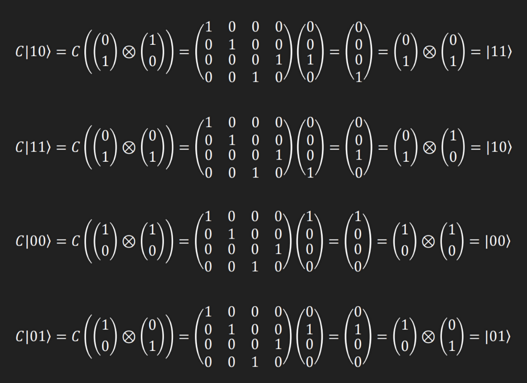
This operation can also be represented as a matrix.
\[ C = \begin{pmatrix} 1 & 0 & 0 & 0 \\ 0 & 1 & 0 & 0 \\ 0 & 0 & 0 & 1 \\ 0 & 0 & 1 & 0 \\ \end{pmatrix} \]
Note how the operations in 2.4 and 2.5 were expressed as matrices. In the quantum world, where probability reigns, the only way to perform deterministic operations is to multiply an unobserved qbit by a matrix. In the example below, the one thing we can be certain of is that the probabilities of observing 0 and 1 have been swapped.
\[ \begin{pmatrix} 0 & 1 \\ 1 & 0 \end{pmatrix} \begin{pmatrix} \frac{1}{2} \\ \frac{\sqrt{3}}{2} \end{pmatrix} = \begin{pmatrix} \frac{\sqrt{3}}{2} \\ \frac{1}{2} \end{pmatrix} \]
Of course, if we only use \(\mid0\rangle\) or \(\mid1\rangle\), which always collapse to 0 or 1, we wouldn't need matrix operations at all -- but then we'd just be using a classical computer. There would be no reason to maintain the extreme conditions near 0K required for quantum computation.
So matrix operations are critical in quantum computing. There's one additional constraint: the matrices used must be reversible. This means that the Constant-0 and Constant-1 operations from the 1-bit operations above cannot be computed by simple matrix multiplication -- a different approach is needed.
The Deutsch-Jozsa problem
This problem[1] is a very simple (and simultaneously
useless) problem that demonstrates a computational advantage
of quantum computers over classical ones.
Suppose there is a function that takes a 1-bit input and produces a 1-bit output. To determine whether this function is constant (Constant-0 or Constant-1) or balanced (Identity or Negation), what is the minimum number of queries required?
Classical computer
A classical computer must test both 0 and 1 as inputs, so it requires two queries.
Quantum computer
As you might expect, the answer is one. To see why, we need a few more concepts.
Hadamard gate
This is the H gate mentioned earlier.
\[ H = \begin{pmatrix} \frac{1}{\sqrt{2}} & \frac{1}{\sqrt{2}} \\ \frac{1}{\sqrt{2}} & \frac{-1}{\sqrt{2}} \end{pmatrix} \]
The Hadamard gate takes a 0- or 1-qbit and transforms it into a qbit with equal probability of being 0 or 1.
\[ H\mid0\rangle = \begin{pmatrix} \frac{1}{\sqrt{2}} & \frac{1}{\sqrt{2}} \\ \frac{1}{\sqrt{2}} & \frac{-1}{\sqrt{2}} \end{pmatrix} \begin{pmatrix} 1 \\ 0 \end{pmatrix} = \begin{pmatrix} \frac{1}{} \\ \frac{1}{\sqrt{2}} \end{pmatrix} \]
\[ H\mid1\rangle = \begin{pmatrix} \frac{1}{\sqrt{2}} & \frac{1}{\sqrt{2}} \\ \frac{1}{\sqrt{2}} & \frac{-1}{\sqrt{2}} \end{pmatrix} \begin{pmatrix} 0 \\ 1 \end{pmatrix} = \begin{pmatrix} \frac{1}{} \\ \frac{-1}{\sqrt{2}} \end{pmatrix} \]
The Hadamard gate has another important property: it sends a qbit with equal probability of 0 and 1 back to a definite 0- or 1-qbit.
\[ \begin{pmatrix} \frac{1}{\sqrt{2}} & \frac{1}{\sqrt{2}} \\ \frac{1}{\sqrt{2}} & \frac{-1}{\sqrt{2}} \end{pmatrix} \begin{pmatrix} \frac{1}{\sqrt{2}} \\ \frac{1}{\sqrt{2}} \end{pmatrix} = \begin{pmatrix} 1 \\ 0 \end{pmatrix} \]
\[ \begin{pmatrix} \frac{1}{\sqrt{2}} & \frac{1}{\sqrt{2}} \\ \frac{1}{\sqrt{2}} & \frac{-1}{\sqrt{2}} \end{pmatrix} \begin{pmatrix} \frac{1}{\sqrt{2}} \\ \frac{-1}{\sqrt{2}} \end{pmatrix} = \begin{pmatrix} 0 \\ 1 \end{pmatrix} \]
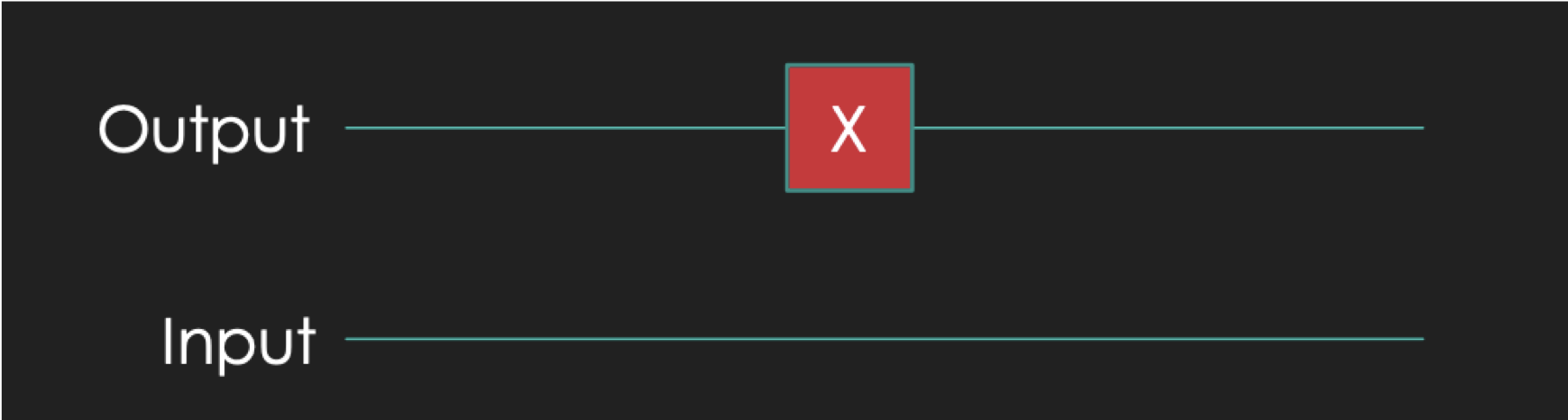
X gate
The X gate swaps the top and bottom components of a qbit.
\[ X = \begin{pmatrix} 0 & 1 \\ 1 & 0 \end{pmatrix} \]
\[ \begin{pmatrix} 0 & 1 \\ 1 & 0 \end{pmatrix} \begin{pmatrix} 0 \\ 1 \end{pmatrix} = \begin{pmatrix} 1 \\ 0 \end{pmatrix} \]
\[ \begin{pmatrix} 0 & 1 \\ 1 & 0 \end{pmatrix} \begin{pmatrix} \frac{-1}{\sqrt{2}} \\ \frac{1}{\sqrt{2}} \end{pmatrix} = \begin{pmatrix} \frac{1}{\sqrt{2}} \\ \frac{-1}{\sqrt{2}} \end{pmatrix} \]
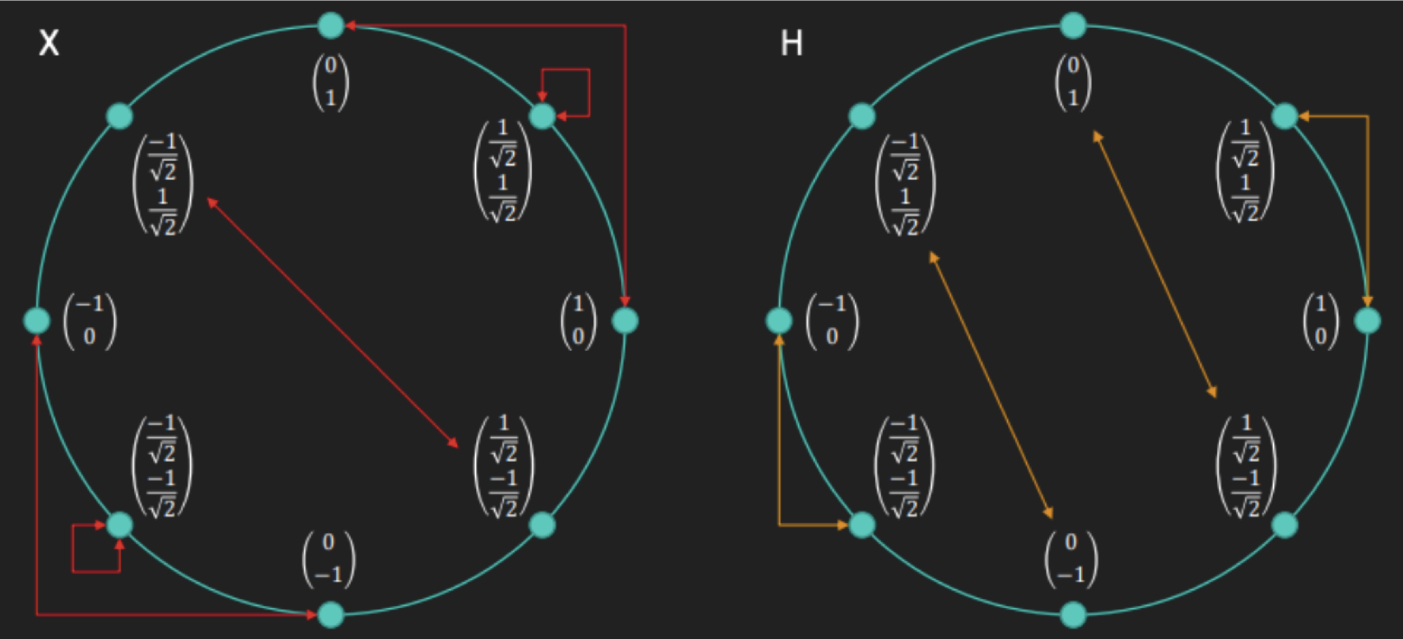
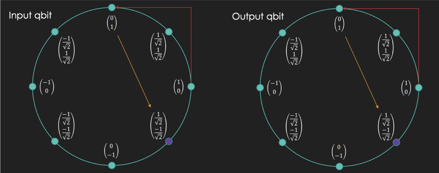
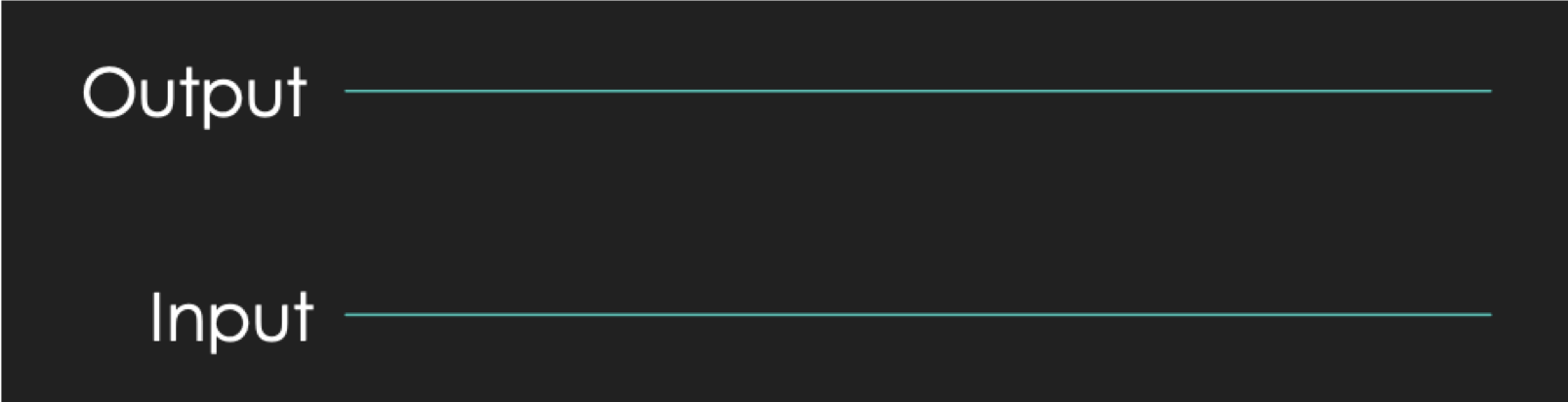
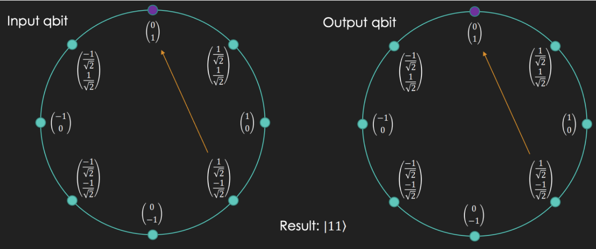
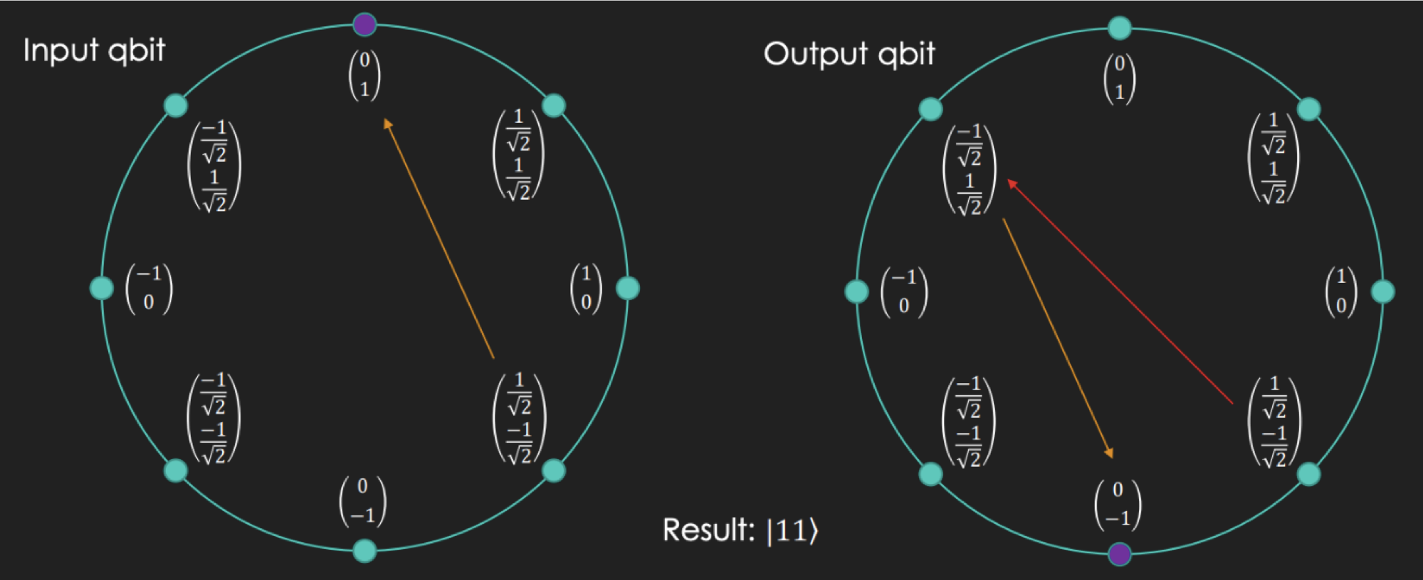
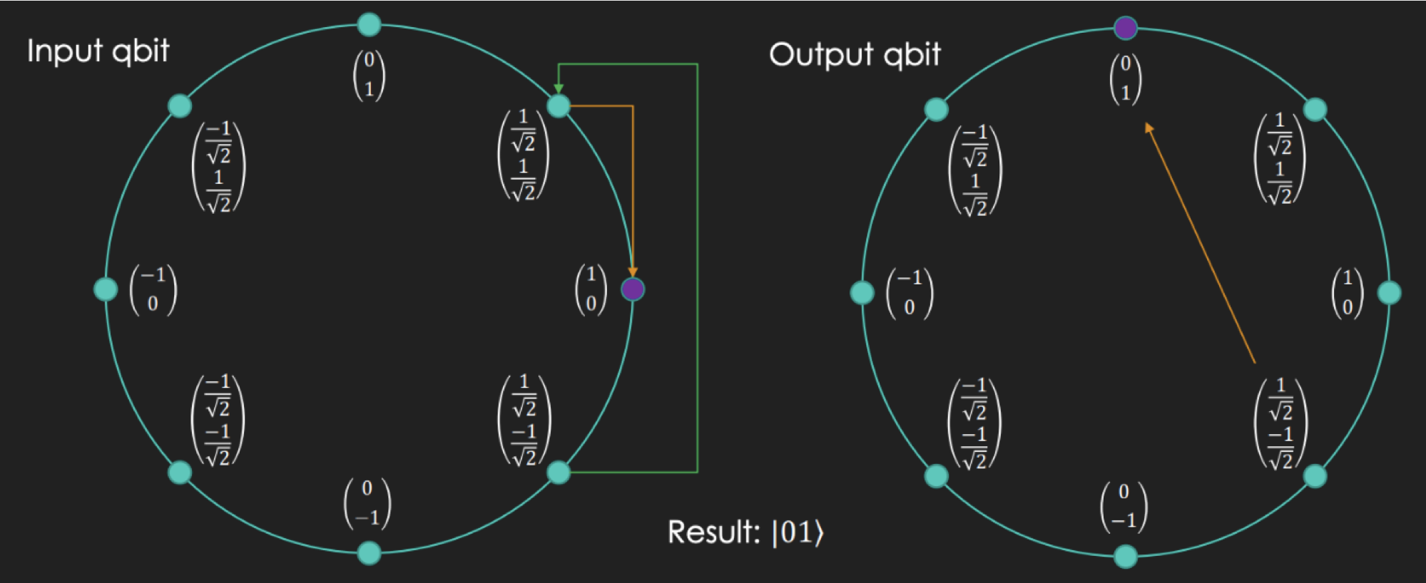
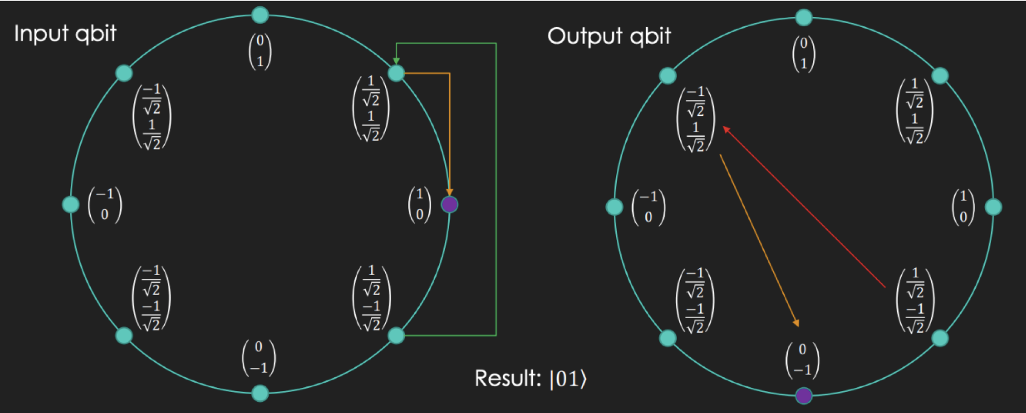
The H gate and X gate operations are easier to understand with the diagram below. Red indicates the X gate and yellow indicates the H gate direction.
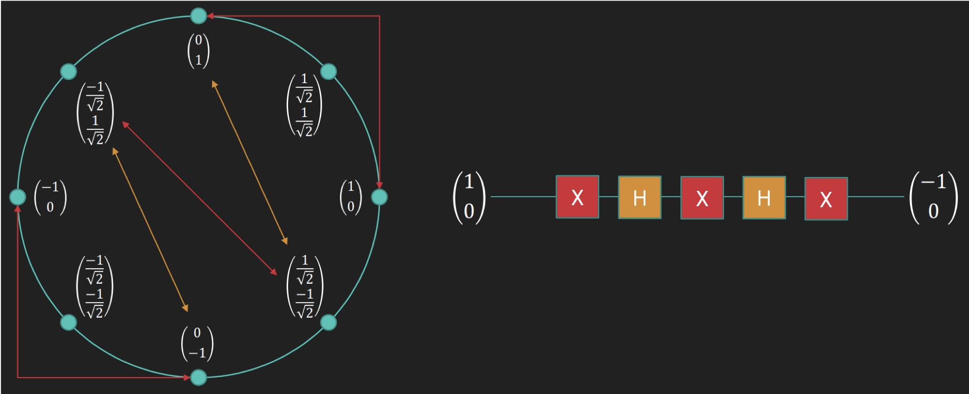
The result of applying X - H - X - H - X gates to \(\begin{pmatrix} 1 \\ 0 \end{pmatrix}\) is much easier to follow in the diagram. Starting from \(\begin{pmatrix} 1 \\ 0 \end{pmatrix}\), follow the arrows in the direction of each gate -- where you end up is the result.
non-reversible matrix
Earlier I mentioned that quantum computers cannot multiply by non-reversible matrices. Among the 1-bit operations, Constant-0 and Constant-1 are non-reversible. To handle these in quantum computing, we use two qbits.
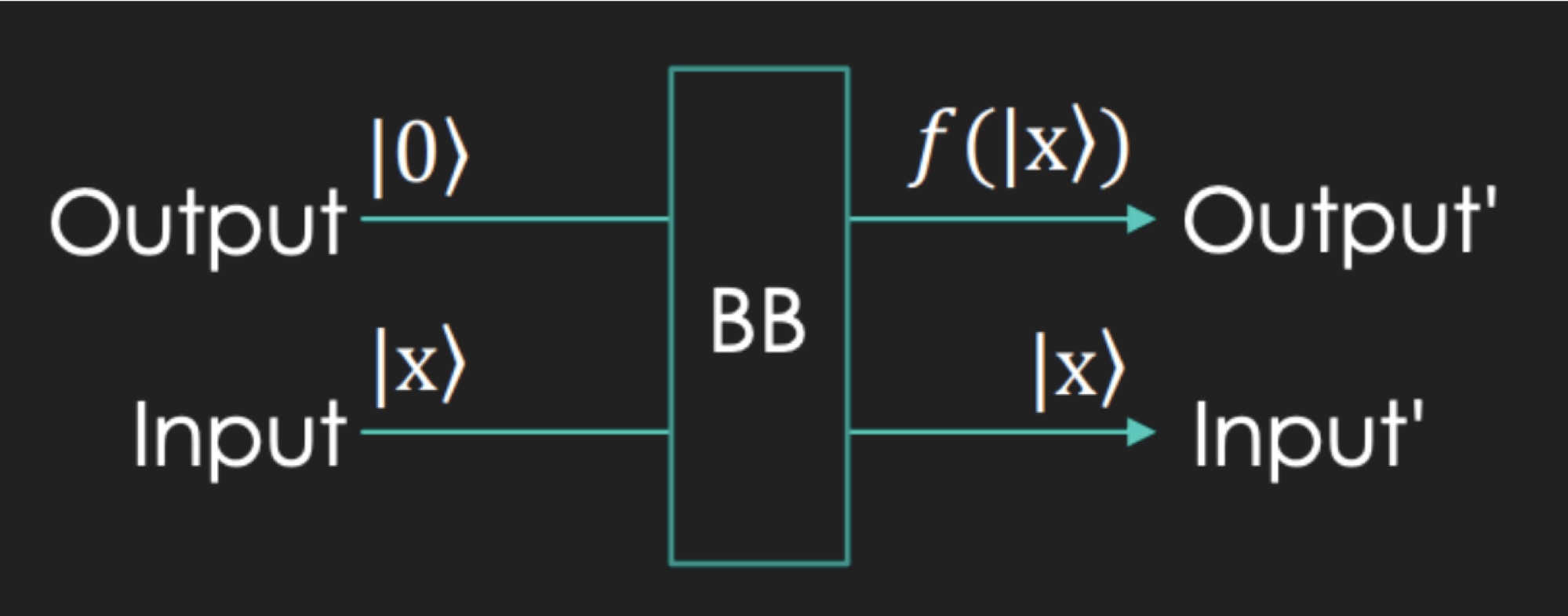
The notation looks backwards at first. Input' and
Output' represent the actual 1-bit operation's input and
output. Input and Output are what we feed in
before the black box (BB) so that Input' and
Output' -- which appear after BB -- land on the
right values. They exist because every quantum operation must be
reversible.
Some examples make this clearer.
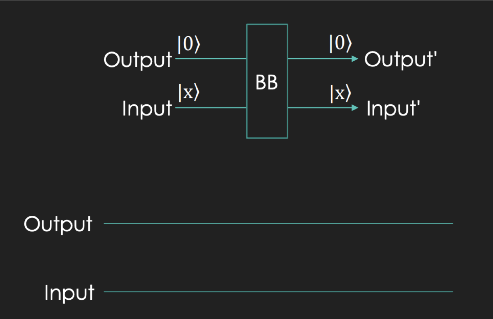
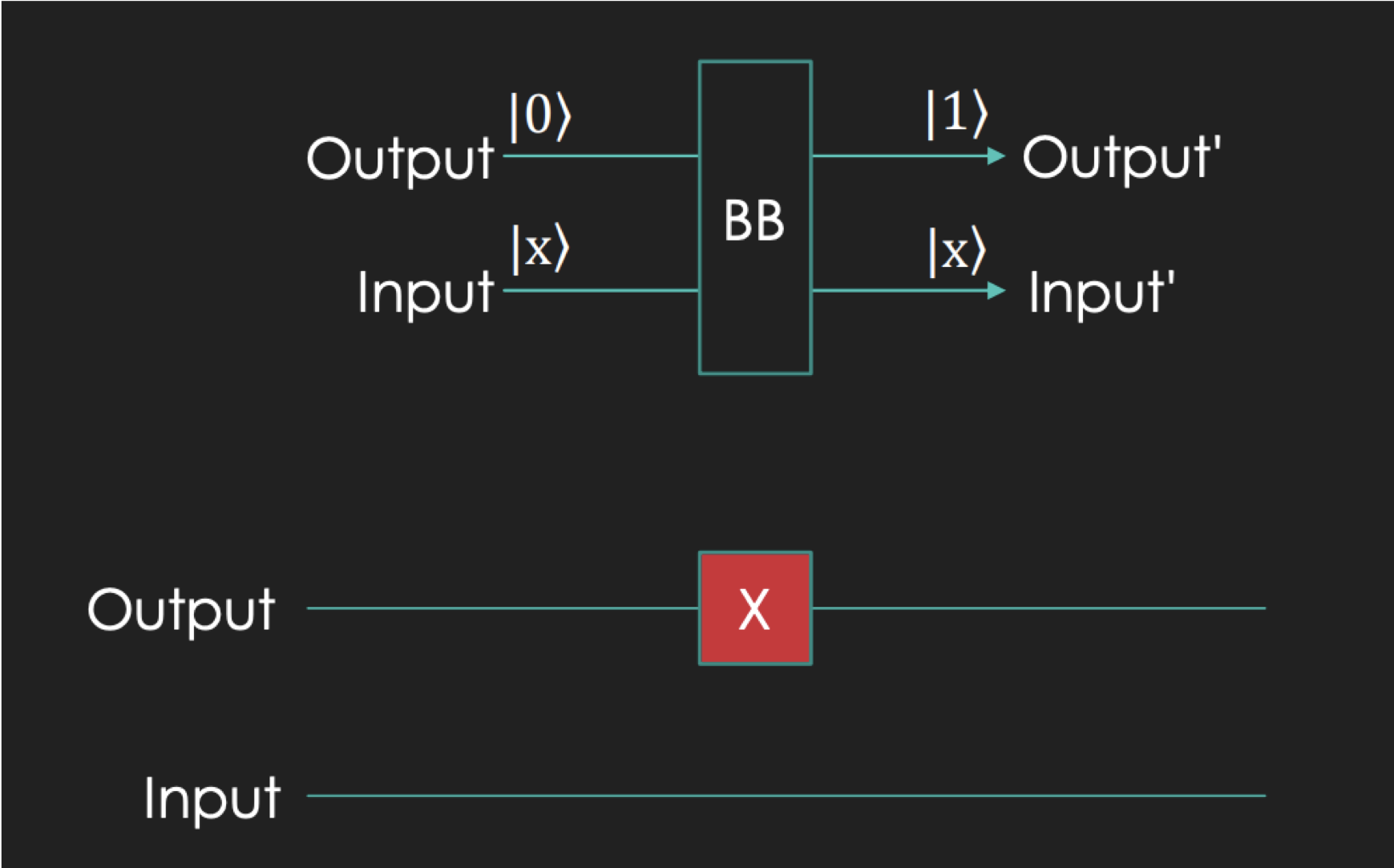

For Constant-0, Output' must be \(\mid 0 \rangle\)
regardless of whether Input' is \(\mid 0 \rangle\) or
\(\mid 1 \rangle\). In the upper-left circuit (which has no gates),
substituting \(\mid 0 \rangle\) or \(\mid 1 \rangle\) into
Input confirms that Input' and
Output' satisfy the Constant-0 relationship.
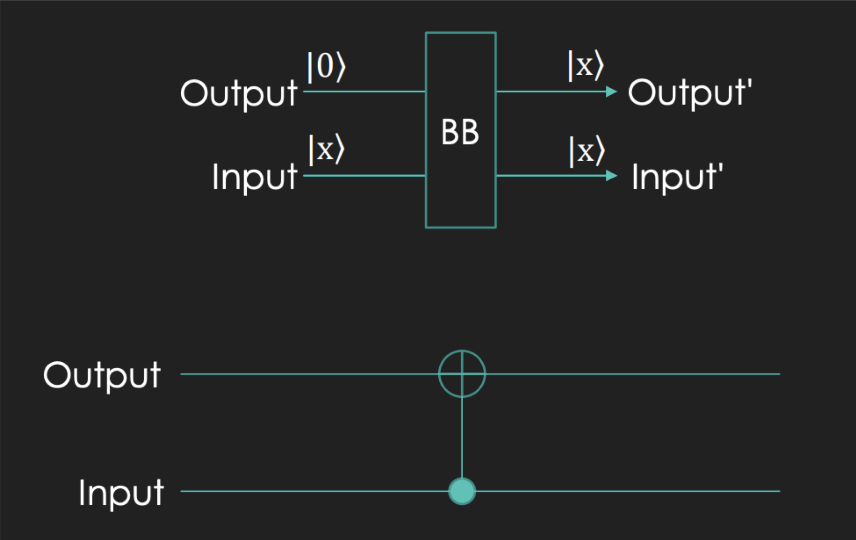
Identity means Output' equals \(\mid 0 \rangle\) when
Input' is \(\mid 0 \rangle\), and Output'
equals \(\mid 1 \rangle\) when Input' is \(\mid 1
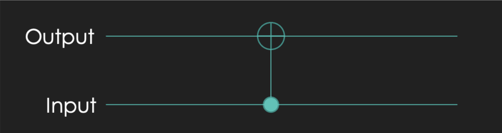
\rangle\). The lower-left circuit represents a CNOT gate: the filled
circle marks the control bit, and the open circle marks the target bit.
If Input is \(\mid 0 \rangle\), the control bit is 0, so
the target bit stays unchanged -- both Input' and
Output' are \(\mid 0 \rangle\). If Input is
\(\mid 1 \rangle\), the control bit is 1, so the target bit flips --
both Input' and Output' become \(\mid 1
\rangle\).
Now let's return to the Deutsch-Jozsa problem: how can a quantum computer solve it in a single query? The answer is captured in the diagram below.
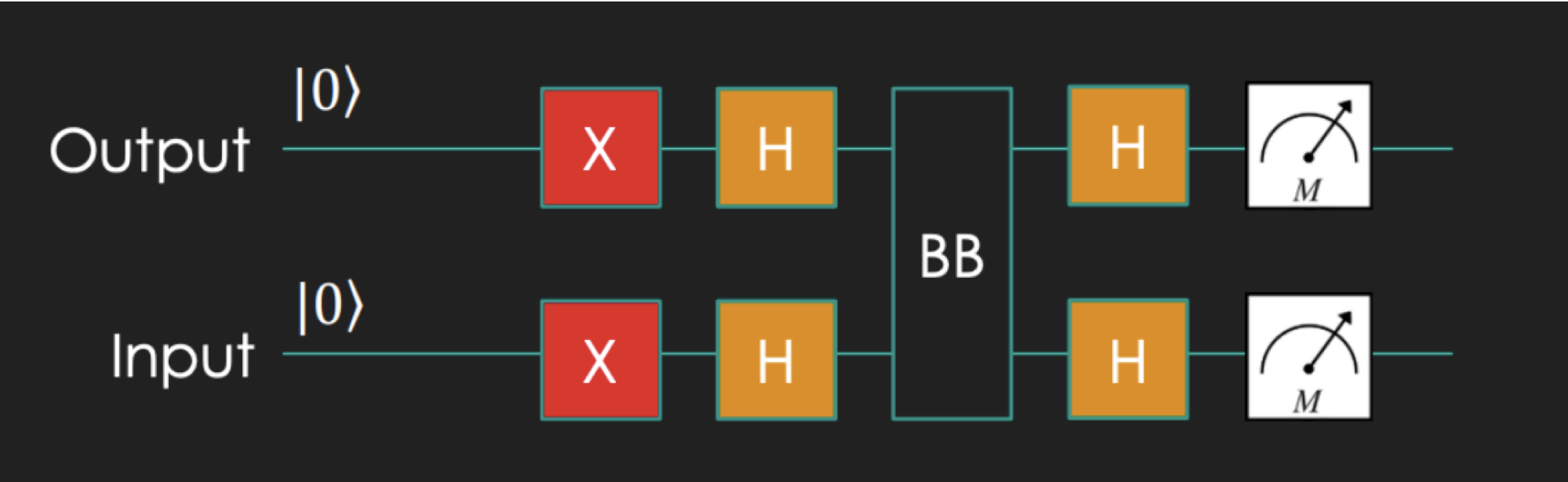
With this circuit, if BB was constant (Constant-0 or Constant-1), the measurement yields \(\mid11\rangle\), and if BB was balanced (Identity or Negation), the measurement yields \(\mid01\rangle\).
Let's walk through each possible BB case to see why.
preprocessing (operations before BB)
Before entering BB, both the input (\(\mid 0 \rangle\)) and output qbit (\(\mid 0 \rangle\)) pass through an X gate followed by an H gate, resulting in \(\begin{pmatrix} \frac{1}{\sqrt{2}} \\ \frac{-1}{\sqrt{2}} \end{pmatrix}\).
case 1) BB is Constant-0
Constant-0 applies no gates to the input or output. So when BB is Constant-0, the Input and Output simply pass through the final H gate before being measured.
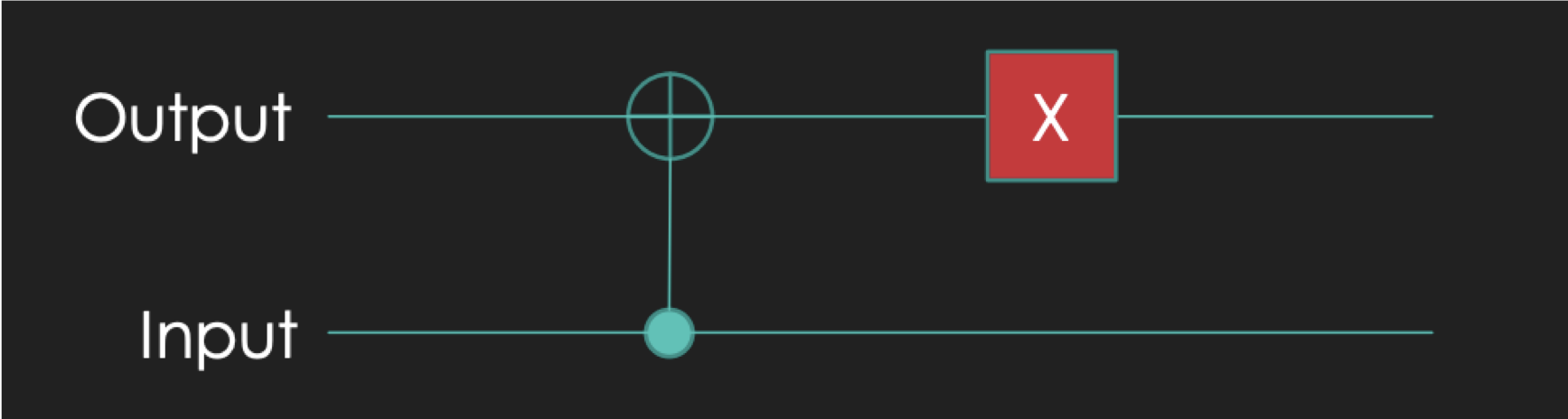
case 2) BB is Constant-1
Constant-1 applies an X gate only to the output. So when BB is Constant-1, an X gate is added to the Output, and then H gates are applied to both Input and Output.
case 3) BB is Identity
Identity is computed using a CNOT gate. As shown earlier, the CNOT operation is equivalent to multiplying by \( \begin{pmatrix} 1 & 0 & 0 & 0 \\ 0 & 1 & 0 & 0 \\ 0 & 0 & 0 & 1 \\ 0 & 0 & 1 & 0 \\ \end{pmatrix} \). After preprocessing, both Input and Output are \( \begin{pmatrix} \frac{1}{\sqrt{2}} \\ \frac{-1}{\sqrt{2}} \end{pmatrix} \), so the CNOT operation can be written as:
\[ C \begin{pmatrix} \begin{pmatrix} \frac{1}{\sqrt{2}} \\ \frac{-1}{\sqrt{2}} \end{pmatrix} \otimes \begin{pmatrix} \frac{1}{\sqrt{2}} \\ \frac{-1}{\sqrt{2}} \end{pmatrix} \end{pmatrix} = C \begin{pmatrix} \frac{1}{2} \\ \frac{-1}{2} \\ \frac{-1}{2} \\ \frac{1}{2} \end{pmatrix} = \frac{1}{2} \begin{pmatrix} 1 & 0 & 0 & 0 \\ 0 & 1 & 0 & 0 \\ 0 & 0 & 0 & 1 \\ 0 & 0 & 1 & 0 \\ \end{pmatrix} \begin{pmatrix} 1 \\ -1 \\ -1 \\ 1 \end{pmatrix} = \frac{1}{2} \begin{pmatrix} 1 \\ -1 \\ 1 \\ -1 \end{pmatrix} = \begin{pmatrix} \frac{1}{\sqrt{2}} \\ \frac{1}{\sqrt{2}} \end{pmatrix} \otimes \begin{pmatrix} \frac{1}{\sqrt{2}} \\ \frac{-1}{\sqrt{2}} \end{pmatrix} \]
So Input changes from \( \begin{pmatrix} \frac{1}{\sqrt{2}} \\ \frac{-1}{\sqrt{2}} \end{pmatrix} \) to \( \begin{pmatrix} \frac{1}{\sqrt{2}} \\ \frac{1}{\sqrt{2}} \end{pmatrix}\), while Output remains \( \begin{pmatrix} \frac{1}{\sqrt{2}} \\ \frac{-1}{\sqrt{2}} \end{pmatrix} \). After the final H gate is applied to each, the result is \(\mid 01 \rangle\).
case 4) BB is Negation
Negation is the Identity result with an additional X gate applied only to the Output. So the computation proceeds as shown below, and just like Identity, the final result is \(\mid 01 \rangle\).
In summary, given the right circuit design, a quantum computer only needs one measurement to determine whether BB is constant or balanced.
Entanglement
The CNOT gate in the Deutsch-Jozsa circuit hints at something deeper. When certain gate combinations act on multiple qbits, the result can't be separated back into individual qbits. That's entanglement.
\( \begin{pmatrix} \frac{1}{\sqrt{2}} \\ 0 \\ 0 \\ \frac{1}{\sqrt{2}} \end{pmatrix} \) is an entangled qbit state. It looks similar to a product state, but differs in one crucial way. As explained above, a product state can be factored into individual qbits. An entangled state cannot. (If the product state of two qbits cannot be factored, they are said to be entangled.) Because of this, an entangled qbit pair behaves as a single unit -- measuring part of it immediately tells you the state of the rest.
Proving that \( \begin{pmatrix} \frac{1}{\sqrt{2}} \\ 0 \\ 0 \\ \frac{1}{\sqrt{2}} \end{pmatrix} \) is entangled is straightforward. Since there are no values \(a\), \(b\), \(c\), \(d\) that satisfy \( \begin{pmatrix} \frac{1}{\sqrt{2}} \\ 0 \\ 0 \\ \frac{1}{\sqrt{2}} \end{pmatrix} = \begin{pmatrix} a \\ b \end{pmatrix} \otimes \begin{pmatrix} c \\ d \end{pmatrix} \), this is an entangled state.
Entangled qbits can be easily created using a CNOT gate and an H gate.
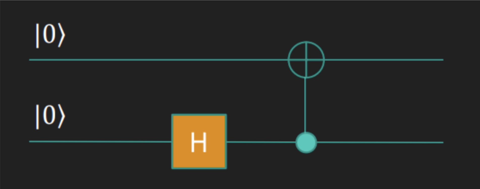
\[ CH_1 \begin{pmatrix} \begin{pmatrix} 1 \\ 0 \end{pmatrix} \otimes \begin{pmatrix} 1 \\ 0 \end{pmatrix} \end{pmatrix} = C \begin{pmatrix} \begin{pmatrix} \frac{1}{\sqrt{2}} \\ \frac{1}{\sqrt{2}} \end{pmatrix} \otimes \begin{pmatrix} 1 \\ 0 \end{pmatrix} \end{pmatrix} = \begin{pmatrix} 1 & 0 & 0 & 0 \\ 0 & 1 & 0 & 0 \\ 0 & 0 & 0 & 1 \\ 0 & 0 & 1 & 0 \\ \end{pmatrix} \begin{pmatrix} \frac{1}{\sqrt{2}} \\ 0 \\ \frac{1}{\sqrt{2}} \\ 0 \end{pmatrix} = \begin{pmatrix} \frac{1}{\sqrt{2}} \\ 0 \\ 0 \\ \frac{1}{\sqrt{2}} \end{pmatrix} \]
This is the same H + CNOT pattern that appears in the Deutsch-Jozsa circuit. Entanglement is doing work there even when it isn't the point.
Conclusion
The thing that surprised me most: quantum supremacy doesn't just happen. The Deutsch-Jozsa circuit works because someone designed the right sequence of H gates and CNOT operations to extract a global property in one shot. Quantum advantage is engineered, not inherent.
I still don't know what a qbit looks like physically, or how gates
are applied to actual hardware. But I now understand why a
quantum computer can answer in one query what a classical computer needs
two for. That feels like enough for a Hello World!.